LECTURE -9 CREATING A CHART IN MICROSOFT EXCEL. CHARTS Picture representation of data used Easy understanding Comparison of data Checking trends in data.

Presentation on theme: "LECTURE -9 CREATING A CHART IN MICROSOFT EXCEL. CHARTS Picture representation of data used Easy understanding Comparison of data Checking trends in data."— Presentation transcript:

1 LECTURE -9 CREATING A CHART IN MICROSOFT EXCEL

2 CHARTS Picture representation of data used Easy understanding Comparison of data Checking trends in data In Excel along with worksheets, worksheet data can be shown in picture representation or statically graph can be created for the data in the worksheet.

3 CREATING A CHARTS OR GRAPH Types of charts

4 COLUMN CHARTS Data that is arranged in columns or rows on a worksheet can be plotted in a column chart. Column charts are useful for showing data changes over a period of time or for illustrating comparisons among items. In column charts, categories are typically organized along the horizontal axis and values along the vertical axis.

5 LINE CHARTS Data that is arranged in columns or rows on a worksheet can be plotted in a line chart. Line charts can display continuous data over time, set against a common scale use a line chart if your category labels are text, and are representing evenly spaced values such as months, quarters or trade and business years

6 PIE CHARTS Data that is arranged in one column or row only on a worksheet can be plotted in a pie chart. Simple Pie charts have only one data series proportional to the sum of the items.. in a pie chart are displayed as a percentage of the whole pie.

7 BAR CHARTS Data that is arranged in columns or rows on a worksheet can be plotted in a bar chart. Bar charts illustrate comparisons among individual items. Consider using a bar chart when: The axis labels are long. The values that are shown are durations

8 STEP 1: On the worksheet, arrange the data that you want to plot in a chart

9 STEP 2: Select the cells that contain the data that you want to use for the chart.

10 STEP 3: On the Insert tab, in the Charts group, select the chart type that you want to use. 1 2 3

11 STEP 4: By default,the chart is placed on the worksheet.

12 STEP 5: If you want to place the chart in a separate chart sheet: Click on the chart Click the Design menu Click the Move Chart button Choose New sheet

13 STEP 6: You can change the chart type by clicking on the chart type from Insert menu 1 2 2

14 STEP 7: You can change the chart design by clicking on the design from the Design menu 1 2

15 STEP 8: To change the chart layout, click on the Layout menu, click on the chart element that you want to change, and then click the layout option that you want. See next slide

16

17 2 3 1 1 2 No gridlines 3

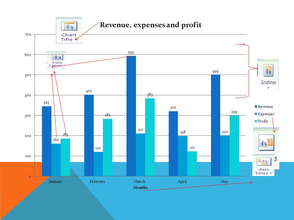
18 -Now.. Use the following buttons to do the following tasks : - Add/remove chart title -Add /remove axis titles -Add/remove data labels -Show or hide a legend -Display or hide chart axes or gridlines -Display or hide primary or secondary axis -Display or hide gridlines

19 EXERCISE: Enter the following data into an Excel worksheet: MonthsRevenueExpensesProfit January345160 February402120 March593210 April320198 May499200 June450250

20 Calculate the profit using this formula (profit = revenue – expenses) Calculate the average for : revenue, expenses and profit. Place the result below each column. Create a column chart for revenue, expenses and profit and save in new worsheet with ‘ column chart ‘ as name Create a pie chart for months and profit. Save the pie chart in a new worksheet as ‘pie chart’ Note : Format your charts so they should look like the charts on the next slide,

21

22